Plot UMAP or embeddings

Plot one or more features by coloring cells in a UMAP plot.

Usage

plot_embedding(
  source,
  embedding,
  features = NULL,
  quantile_range = c(0.01, 0.99),
  randomize_order = TRUE,
  smooth = NULL,
  smooth_rounds = 3,
  gene_mapping = human_gene_mapping,
  size = NULL,
  rasterize = FALSE,
  raster_pixels = 512,
  legend_continuous = c("auto", "quantile", "value"),
  labels_quantile_range = TRUE,
  colors_continuous = c("lightgrey", "#4682B4"),
  legend_discrete = TRUE,
  labels_discrete = TRUE,
  colors_discrete = discrete_palette("stallion"),
  return_data = FALSE,
  return_plot_list = FALSE,
  apply_styling = TRUE
)

Arguments

source

Matrix, or data frame to pull features from, or a vector of feature values for a single feature. For a matrix, the features must be rows.

embedding

A matrix of dimensions cells x 2 with embedding coordinates

features

Character vector of features to plot if source is not a vector.

quantile_range

(optional) Length 2 vector giving the quantiles to clip the minimum and maximum color scale values, as fractions between 0 and 1. NULL or NA values to skip clipping

randomize_order

If TRUE, shuffle cells to prevent overplotting biases. Can pass an integer instead to specify a random seed to use.

smooth

(optional) Sparse matrix of dimensions cells x cells with cell-cell distance weights for smoothing.

smooth_rounds

Number of multiplication rounds to apply when smoothing.

gene_mapping

An optional vector for gene name matching with match_gene_symbol(). Ignored if source is a data frame.

size

Point size for plotting

rasterize

Whether to rasterize the point drawing to speed up display in graphics programs.

raster_pixels

Number of pixels to use when rasterizing. Can provide one number for square dimensions, or two numbers for width x height.

legend_continuous

Whether to label continuous features by quantile or value. "auto" labels by quantile only when all features are continuous and quantile_range is not NULL. Quantile labeling adds text annotation listing the range of displayed values.

labels_quantile_range

Whether to add a text label with the value range of each feature when the legend is set to quantile

colors_continuous

Vector of colors to use for continuous color palette

legend_discrete

Whether to show the legend for discrete (categorical) features.

labels_discrete

Whether to add text labels at the center of each group for discrete (categorical) features.

colors_discrete

Vector of colors to use for discrete (categorical) features.

return_data

If true, return data from just before plotting rather than a plot.

return_plot_list

If TRUE, return multiple plots as a list, rather than a single plot combined using patchwork::wrap_plots()

apply_styling

If false, return a plot without pretty styling applied

Value

By default, returns a ggplot2 object with all the requested features plotted in a grid. If return_data or return_plot_list is called, the return value will match that argument.

Details

Smoothing

Smoothing is performed as follows: first, the smoothing matrix is normalized so the sum of incoming weights to every cell is 1. Then, the raw data values are repeatedly multiplied by the smoothing matrix and re-scaled so the average value stays the same.

Examples

set.seed(123)
mat <- get_demo_mat()
## Normalize matrix
mat_norm <- log1p(multiply_cols(mat, 1/colSums(mat)) * 10000) %>% write_matrix_memory(compress = FALSE)
## Get variable genes
stats <- matrix_stats(mat, row_stats = "variance")
variable_genes <- order(stats$row_stats["variance",], decreasing=TRUE) %>% 
  head(1000) %>% 
  sort()
# Z score normalize genes
mat_norm <- mat[variable_genes, ]
gene_means <- stats$row_stats['mean', variable_genes]
gene_vars <- stats$row_stats['variance', variable_genes]
mat_norm <- (mat_norm - gene_means) / gene_vars
## Save matrix to memory
mat_norm <- mat_norm %>% write_matrix_memory(compress = FALSE)
## Run SVD
svd <- BPCells::svds(mat_norm, k = 10)
pca <- multiply_cols(svd$v, svd$d)
## Get UMAP
umap <- uwot::umap(pca)
## Get clusters
clusts <- knn_hnsw(pca, ef = 500) %>%
  knn_to_snn_graph() %>%
  cluster_graph_louvain()
#> 17:37:39 Building HNSW index with metric 'euclidean' ef = 200 M = 16 using 1 threads
#> 17:37:39 Finished building index
#> 17:37:39 Searching HNSW index with ef = 500 and 1 threads
#> 17:37:39 Finished searching


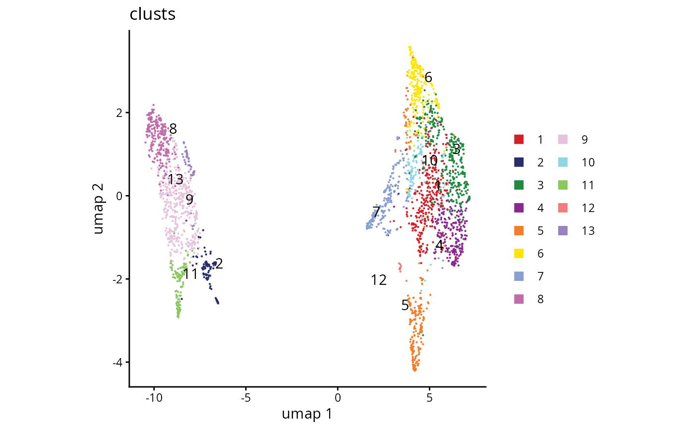
## Plot embedding
print(length(clusts))
#> [1] 2600

plot_embedding(clusts, umap)
#> Error in names(x) <- value: 'names' attribute [175] must be the same length as the vector [1]


### Can also plot by features
#plot_embedding(
#  source = mat,
#  umap,
#  features = c("MS4A1", "CD3E"),
#)